Research Article | | Peer-Reviewed

Spatial Modeling of Cardiovascular Disease in Kenya

Received: 20 March 2026     Accepted: 3 April 2026     Published: 16 April 2026
Views:       Downloads:
Abstract

The study conducts an assessment of the spatial distribution of cardiovascular diseases (CVD) in Kenya by integrating spatial modeling techniques and spatial autocorrelation measures. CVDs, which refer to disorders of the heart and blood vessels, have surpassed communicable diseases as the leading cause of morbidity and mortality worldwide, posing a critical public health concern, especially in low- and middle-income countries (LMICs) where resources remain limited. A growing body of global evidence has revealed marked geographical disparities in CVD incidence, prompting investigations into small-area spatial distribution patterns. This study employed both global and local spatial autocorrelation measures to analyze CVD prevalence across Kenyan counties. The Global Moran’s I statistic was used to assess the overall degree of spatial clustering, while the Local Moran’s I identified significant clusters of high and low prevalence, alongside spatial outliers. Additionally, the Getis-Ord Gi* statistic was applied to detect statistically significant hotspots and coldspots, revealing important spatial patterns in disease prevalence. Spatial regression models were compared using the Lagrange Multiplier (LM) test, Akaike Information Criterion (AIC), and Bayesian Information Criterion (BIC) for model selection. The Spatial Lag Model (SLM) demonstrated superior performance over the Spatial Error Model (SEM) and the Spatial Durbin Model (SDM), achieving a Rao’s score (RSlag) of 16.449 and an adjusted score (adjRSlag) of 12.181, both statistically significant at the 5% level. The SLM also recorded the lowest AIC and BIC values at -380.09 and -361.80, respectively, confirming its suitability in capturing spatial dependence in the data. The findings revealed significant spatial clustering of CVD prevalence, with distinct high-risk and low-risk regions across the country. High body mass index (HBMI), tobacco use, and poor dietary habits emerged as major risk factors driving CVD prevalence, while urbanization and economic development were associated with lower disease burdens. The study highlights the importance of incorporating spatial analysis in public health planning to inform targeted interventions, optimize resource allocation, and enhance community health education campaigns aimed at promoting heart-healthy lifestyles.

Published in American Journal of Theoretical and Applied Statistics (Volume 15, Issue 2)
DOI 10.11648/j.ajtas.20261502.14
Page(s) 59-71
Creative Commons

This is an Open Access article, distributed under the terms of the Creative Commons Attribution 4.0 International License (http://creativecommons.org/licenses/by/4.0/), which permits unrestricted use, distribution and reproduction in any medium or format, provided the original work is properly cited.

Copyright

Copyright © The Author(s), 2026. Published by Science Publishing Group

Keywords

Cardiovascular Diseases (CVDS), Global Moran’s I, Local Moran’s I, Spatial Lag Model (SLM), Spatial Error Model (SEM), Spatial Durbin Model (SDM), Gertis Ord Gi* Statistic

1. Introduction
Cardiovascular diseases (CVDs) refer to disorders of the heart and blood vessels, including ischemic heart disease, stroke, peripheral arterial disease, rheumatic heart disease, congenital heart disease, deep vein thrombosis, and pulmonary embolism . These diseases are a leading cause of morbidity and mortality globally, contributing to approximately 17.8 million deaths annually with the majority of these deaths, nearly 80%, occurring in low and middle-income countries (LMIC) including Kenya . In Kenya, CVDs are increasingly recognized as a significant public health challenge rapidly overshadowing the infectious diseases that once dominated the health landscape, contributing to premature deaths and straining an already overburdened healthcare system.
Multiple risk factors for non-communicable diseases have contributed to the rising prevalence of cardiovascular disease (CVD) in Kenya. The 2015 STEPwise survey for noncommunicable disease risk factors in Kenya highlighted widespread exposure to CVD risk factors, including elevated blood pressure, tobacco use, physical inactivity, unhealthy dietary habits, and excess body weight . These factors collectively fuel the growing burden of CVD, placing significant pressure on the country’s healthcare system and economy.
Despite national efforts through NCD strategic plans, the scarcity of studies examining the spatial patterns and disparities of CVD in Kenya has led to lack of a national strategy that prioritizes CVDs , limiting the ability to guide targeted interventions and allocate resources effectively. Advancements in spatial analysis techniques offer opportunities to uncover geographic patterns of disease distribution. Spatial regression and hotspot analysis methods can detect spatial autocorrelation, identify disease clusters, and model the relationships between CVD prevalence across counties.
A review of existing literature highlights the significance of this study in integrating non-spatial epidemiological approaches with advanced spatial modelling techniques in the analysis of CVDs . Although numerous studies have employed conventional statistical methods to examine CVD prevalence and associated risk factors, the application of spatial autoregressive models and hotspot analysis remains comparatively limited, especially in low- and middle-income countries.
This study addresses this methodological gap by identifying spatial dependencies, quantifying regional disparities, and detecting spatial clustering patterns in CVD distribution in Kenya. The findings offer valuable insights for public health policy and planning, providing a spatially explicit, data-driven framework to enhance reduction in morbidity and mortality, optimize the targeting of health interventions, and inform the equitable allocation of healthcare resources aimed at reducing the burden of CVD.
2. Methodology
2.1. Variables and Data Source
Kenya, the study area, is made up of 47 counties, each characterized by diverse demographic, economic, and environmental conditions that shape health outcomes, particularly with regard to cardiovascular disease (CVD).
This study employs the Spatial model to analyze secondary data obtained from the Global Burden of Disease (GBD) 2021 dataset and the 2019 national census data . The GBD 2021 dataset offers detailed information on the prevalence of cardiovascular diseases (CVDs) and associated risk factors across different regions at both national and county levels. The county-level prevalence rate of cardiovascular disease is the dependent variable of this study. Specific risk factors considered include high body mass index (HBMI), high alcohol use, tobacco use, and dietary risks. Meanwhile, the 2019 national census data provides essential demographic and socioeconomic variables, enriching the spatial analysis by offering critical context for adjusting the spatial distribution of CVD burden. Key demographic variables include the urbanization rate and the population density per km2. However, the socioeconomic variable included was the gross county product (GCP).
2.2. Spatial Autocorrelation
Spatial autocorrelation is used to describe the extent to which a variable is correlated with itself through space . The spatial autocorrelation statistic captures both the attribute similarity and the locational similarity. The presence of spatial autocorrelation can be assessed using the Global Moran’s I index and Geary’s C index. The indices summarize the degree to which similar observations tend to occur near each other over the study area. The Morans I is produced by standardizing the spatial autocovariance by the variance of the data while Geary’s C uses the sum of the squared differences between pairs of data values as its measure of covariation. They both depend on a spatial structural specification such as a spatial weights matrix or a distance related decline function.
2.2.1. Spatial Weights Matrix
A spatial weights matrix W indicates the strength of the potential interaction between spatial areal units . In the study, the spatial structure of units is defined by spatial contiguity, represented through a nxn spatial weights matrix W with binary values.
The binary spatial weights matrix W is defined as:
wij={ 0 otherwise 1 if area i and area j are contiguous(1)
The row-standardized weights matrix Wis given by:
wij*=wijjϵJiwij(2)
where Ji is the set of areal units contiguous with i.
The row-standardized matrix satisfies:
 wij=1 for all ijϵJiX*(3)
The values of wij or the weights for each pair of locations are assigned by some preset rules that define the spatial relations among locations and, therefore, determine the spatial autocorrelation statistics. By convention, wii = 0 for the diagonal elements .
Neighbors can be defined by contiguity in different ways: in Rook contiguity, two locations are considered neighbors if they share a common border or side, while in Queen contiguity, any region that touches either the boundary or a single point of the region i is considered a neighbor.
2.2.2. Global Moran’s I
The study employed the Global Moran’s I index to asseess the presence of spatial autocorrelation in the overall data, which quantifies how similar each region is with its neighbors and averages all these assessments.
The Global Moran’s I takes the form:
I=nijwij(Yi - Ȳ)(Yj - Ȳ)(ijwij)i(Yi - Ȳ)2(4)
where, n is the number of regions, Yi is the observed value of the variable of interest in region i, Yj is the observed value of the variable of interest in region j, and Y¯ is the mean of all observed values. wij are spatial weights that denote the spatial proximity between regions i and j, with wii = 0 and i, j = 1,..., n.
Moran’s I values usually range from -1 to 1. The values significantly above E [I] indicate positive spatial autocorrelation or clustering. This occurs when neighboring regions tend to have similar values. On the other hand, Moran’s I values significantly below E [I] indicate negative spatial autocorrelation or dispersion. This happens when regions that are close to one another tend to have different values. However, the values around E [I] indicate randomness, that is, the absence of spatial pattern.
When the number of regions is sufficiently large, I has a normal distribution and we can assess whether any given pattern deviates significantly from a random pattern by comparing the z-score to the standard normal distribution.
z=I - E(I)Var(I)(5)
An alternative approach to judge significance is Monte Carlo randomization. This method creates random patterns by reassigning the observed values among the areas and calculates the Moran’s I for each of the patterns, providing a randomization distribution for the Moran’s I. If the observed value of Moran’s I lies in the tails of this distribution, the assumption of independence among observations is rejected.
2.3. Hotspot Analysis
2.3.1. Getis-Ord Gi* Statistic
In this study, the Hot Spot Analysis tool was employed to identify spatial clusters of high and low values in the prevalence of cardiovascular disease across regions. The tool calculates the Getis-Ord Gi statistic for each feature in the dataset, generating associated z-scores and p-values that indicate where clusters of statistically significant high or low values occur .
The analysis considers each feature within the context of its neighboring features. While an individual county with a high prevalence value is notable, it is only classified as a statistically significant hot spot if it is also surrounded by other counties with similarly high values. The local sum of a feature and its neighbors is compared to the overall sum of all features in the dataset. A statistically significant hot spot is identified when this local sum differs from the expected value by an amount too large to be attributed to random chance, yielding a high positive z-score.
To account for the potential issue of multiple testing and spatial dependency-where the likelihood of identifying statistically significant results by chance increases with the number of tests-the False Discovery Rate (FDR) correction was applied. This adjustment improves the robustness of the statistical inference, ensuring a more reliable identification of true hot and cold spots within the study area.
This methodology was integral to the spatial analysis conducted in this study, providing critical insights into the geographic clustering patterns of cardiovascular disease prevalence in Kenya. The Getis-Ord local statistic is given as:
Gi*=j=1nwi,jxj-j=1nwi,js(j=1nwi,j)1n-1(6)
where xj is the attribute value for f eature j, wi,j is the spatial weight between feature i and j, and n is equal to the total number of features and:
=j=1nxjn(7)
S=j=1nxj2n - ()2(8)
The Gi statistic is a z-score, so no further calculations are required.
2.3.2. Local Indicators of Spatial Association (LISA)
To assess local spatial association between the prevalence of CVD in each county and those of its neighboring counties, Local Indicators of Spatial Association (LISA) were applied in this study. LISA is specifically designed to measure the degree of significant spatial clustering of similar values around each observation, allowing the identification of localized spatial patterns that may be obscured in global statistics.
A desirable property of LISA is that the sum of its local values across all regions is proportional to the corresponding global measure of spatial autocorrelation. This allows for the decomposition of a global statistic into the contribution of each individual region, providing a more localized understanding of spatial patterns.
In this analysis, local Moran’s I values were computed for each county to detect significant clusters. For the i-th region, the local Moran’s I is defined as:
Ii=n(Yi-Ȳ)jwij(Yj-Ȳ) j(Yj-Ȳ)2,(9)
where wij represents the spatial weight between regions i and j, and Y¯ is the mean of Y, the variable of interest.
Importantly, the global Moran’s I is proportional to the sum of the local Moran’s I values for all regions:
I=1ijwijiIi(10)
To interpret the significance of these local Moran’s I values, associated p-values was generated. These p-values represent the probability of obtaining a local Moransˆ I as extreme as the observed one under the null hypothesis of spatial randomness (no spatial association). This allowed for the identification of regions that are part of statistically significant high-high clusters (hot spots) or low-low clusters (cold spots), as well as spatial outliers.
The p-values were estimated through a permutation approach, in which the observed value at a given region i is held constant while the values at other locations are randomly permuted a large number of times to generate a reference distribution of local Moran’s I. The position of the observed statistic within this simulated distribution determines its statistical significance.
2.4. Spatial Models
The justification for using a spatial model begins with testing for spatial autocorrelation in the residuals of an Ordinary Least Squares (OLS) regression model that estimates the linear relationship between the dependent variable and the explanatory variables. The Moran’s I of the residuals of an OLS is used to assess whether residuals exhibit spatial dependence. A significant Moran’s I result indicates a violation of the OLS assumption of independent errors, necessitating the use of a spatial model to account for spatial dependencies across the geographical space.
Spatial econometrics offers a range of models tailored to different data characteristics and research objectives. Among the most commonly used types of spatial regression models which can be chosen subject to the data or theoretical literature are the spatial lag model (SAR model) and the spatial error model (SEM model) . While the two models provide essential frameworks for understanding spatial relationships, Spatial Durbin Model (SDM) build upon and combine these foundational models .
The SAR model addresses spatial dependencies by incorporating spatial lags of the dependent variable. This approach accounts for autocorrelation among observed variables by modeling equilibrium outcomes that result from spatial and/or social interactions . The Spatial Autoregressive (SAR) model can be defined as:
y=ρWy++ϵ(11)
where:
1) y is an N × 1 vector of the dependent variable,
2) W is an N × N spatial weights matrix,
3) X is an N ×K matrix of k = {1, 2,..., K} covariates,
4) ϵ is an N×1 vector of normally distributed disturbances,
5) β is a K × 1 vector of parameter estimates, and
6) ρ represents the autoregressive scalar parameter.
The Spatial Error Model (SEM) addresses spatial dependence in the error term by incorporating a spatial autoregressive process. In a standard linear regression model, the disturbance term u is typically assumed to be i.i.d. However, in the SEM, u follows a first-order autoregressive (AR) process, analogous to the Markov process in time-series analysis. This implies that the error term for one observation can be influenced by the error terms of neighboring observations, reflecting a spatial spillover effect . The Spatial Error Model (SEM) can be defined as:
where:
y=+u(12)
u=λWu+ϵ(13)
In this model:
1) y represents the dependent variable,
2) X denotes the matrix of exogenous (independent) variables,
3) β represents the coefficients for these exogenous variables,
4) u is the vector of spatially correlated error terms,
5) λ is the spatial autoregressive coefficient, measuring the extent of spatial dependence in the error terms,
6) W is the spatial weights matrix indicating the spatial structure and influence of neighboring observations, and
7) ϵ is a vector of i.i.d. (independently and identically distributed) error terms.
The SEM is particularly useful when spatial dependence is confined to the error term rather than the dependent variable itself. It accounts for unobserved spatial heterogeneity and omitted variables that might be spatially correlated.
The Spatial Durbin Model (SDM) captures both spatial dependence in the dependent variable and the spatial spillovers in the explanatory variables. It combines the spatial autoregressive structure for the dependent variable with the spatial lag specification of the covariates, resulting in a more comprehensive representation of spatial interdependencies . The general form of the SDM is expressed as follows:
y=ρWy++WXθ+ϵ(14)
Where:
1) y is the n × 1 vector of the dependent variable (e.g., prevalence of cardiovascular disease),
2) W is the n × n spatial weights matrix that defines the spatial relationships between regions,
3) X is the n×k matrix of explanatory variables (covariates such as population density, socio-economic factors,
4) etc.),
5) β is the k × 1 vector of coefficients for the explanatory variables,
6) WX is the spatial lag of the explanatory variables, capturing spillover effects from neighboring regions,
7) θ is the k × 1 vector of coefficients for the spatially lagged covariates,
8) ρ is the spatial autoregressive coefficient, indicating the impact of the dependent variable’s spatial lag on the outcome in each region,
9) ϵ is the n×1 vector of errors, assumed to follow a normal distribution with zero mean and constant variance.
2.5. The Analytical Strategy
In spatial econometrics, the specific-to-general approach is commonly used to build models progressively. This approach begins with a basic non-spatial model and and systematically tests for possible misspecifications, such as omitted autocorrelation in the error term or the dependent variable . Through these tests, the model is refined by incorporating necessary spatial components to account for the spatial dependencies in the data .
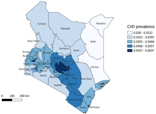
Figure 1. Spatial distribution of Cardiovascular Disease in Kenya.
2.6. Histogram
The Freedman-Diaconis rule has been used to determine the optimal bin width for the histogram. The formula for calculating the width of the bin, h, is given by:
h=2 IQRn1/3
This study begins by conducting an Exploratory Spatial Data Analysis (ESDA) to understand the underlying patterns and distributions in the data. Analysis of spatial autocorrelation of the residuals from the Ordinary Least Squares (OLS) regression is then performed to assess the presence of spatial dependence and justify the use of a spatial model. The Global Moran’s I is computed on the data to detect any overall spatial autocorrelation and determine whether spatial dependence exists across the regions of interest employing the Queen (first order) adjacency weights matrix. The study applies the spatial modelling techniques, namely, spatial lag model, spatial error model, and spatial durbin model. To guide model selection, we will use the Lagrange Multiplier (LM) test and assess model fit through the Akaike Information Criterion (AIC) and Bayesian Information Criterion (BIC). This criterion will enable a comparative evaluation of the relative performance of the spatial models. Once the best model is identified and fit, model diagnostics to ensure the validity of the results is conducted. This includes residual analysis which is essential in assessing the adequacy of fitted spatial model.
3. Results
3.1. Exploratory Spatial Data Analysis
3.1.1. Maps on CVD Prevalence in Kenya
The Natural Breaks (Jenks) classification method effectively reveals inherent data groupings by optimizing class boundaries at points where significant differences in data values occur. This ensures that similar values are grouped while maximizing distinctions between classes. Figure 1 illustrates the spatial distribution of cardiovascular diseases in Kenya and highlight areas with varying concentrations.
where IQR is the interquartile range and n is the number of data points. By focusing on the interquartile range, the Freedman-Diaconis rule reduces the influence of outliers and helps to generate a histogram that accurately represents the data’s central tendency and distribution. Figure 2 shows the distribution of CVDs prevalence using a histogram.
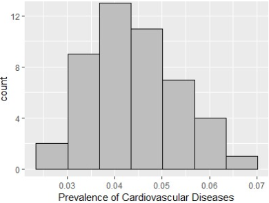
Figure 2. Cardiovascular diseases in Kenya.
3.1.2. Horizontal Bar Graph
Figure 3 shows the CVD distribution using a horizontal bar graph.
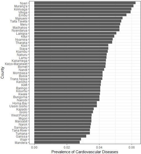
Figure 3. CVD prevalence in the counties across Kenya.
3.1.3. Spatial Lag Scatterplot
Figure 4 shows the scatterplot of the original variable values versus the spatially lagged values.
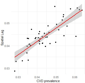
Figure 4. Spatial Lag Scatterplot.
The positive spatial lag scatter plot for the prevalence of cardiovascular disease (CVD) reveals a significant positive correlation, indicating that regions with higher CVD rates tend to be surrounded by neighboring areas with similarly elevated rates.
3.1.4. Residuals from Linear Regression
In Table 1, Moran’s I for the residuals of the OLS regression model is 0.2048, with a z-value of 2.4491 and a significant p-value of 0.0071.
Table 1. Moran’s I for residuals of the OLS regression model.

Disease

Moran’s I

z-value

P-value

Cardiovascular

0.2048

2.4491

0.0071

The significant Moran’s I value suggests that an OLS model would fail to account for key spatial dependencies, necessitating spatial regression techniques.
3.2. Spatial Analysis Results
3.2.1. Global Moran’s I
The results presented in Table 2 highlight the spatial autocorrelation as determined by the global Moran statistic I.
Table 2. Moran’s I Test Results.

Disease

Moran’s I Statistic

p-value

Cardiovascular

0.5875

< 0.001

Stroke

0.5135

< 0.001

Ischemic

0.5598

< 0.001

Rheumatic

0.4057

< 0.001

Hypertensive

0.4985

< 0.001

The statistically significant positive values obtained from the global Moran I test indicate the presence of a positive spatial autocorrelation. This suggests that neighboring areas tend to have high or low prevalence rates of CVD.
3.2.2. Moran’s I Scatterplot
The plot shown in Figure 5 is a Moran’s I scatter plot, which is typically used to assess spatial autocorrelation. It compares the prevalence of cardiovascular disease (CVD) in each region (x-axis) with the prevalence in neighboring regions (y-axis).
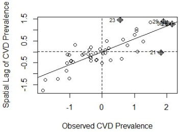
Figure 5. Moran Scatterplot.
The positive slope of the regression line suggests that regions with high (low) CVD prevalence tend to be surrounded by other regions with similarly high (low) CVD prevalence, indicating positive spatial autocorrelation.
3.2.3. Hotspot Analysis
Local Moran’s I have been used in identifying clusters of similar values and highlight spatial outliers, detecting regions where high values cluster with other high values (hotspots), low values cluster with low values (coldspots), and areas where values differ significantly from their neighbors (outliers). In contrast, Getis-Ord Gi* has been used to specifically identify statistically significant hotspots and coldspots, focusing on the concentration of high or low values without detecting outliers. Figure 6 displays the hotspots and coldspots of cardiovascular disease (CVD) prevalence, with hotspots marked in red and coldspots in green. The hotspots indicate regions with higher than-expected CVD prevalence, while coldspots represent areas with lower-than-expected prevalence.
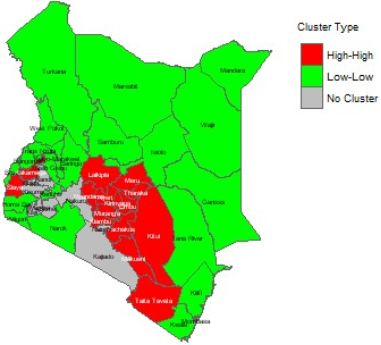
Figure 6. Hotspots and coldspots of CVD in Kenya.
Figure 7 illustrates the significant hotspots and coldspots for cardiovascular disease (CVD) prevalence. It highlights the counties with statistically significant clustering, showing regions with either elevated (hotspots) or reduced (coldspots) CVD prevalence in relation to neighboring areas.
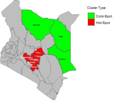
Figure 7. Significant hotspots and coldspots of CVD in Kenya.
The results presented in Tables 3 and 4 summarizes the counties identified as significant hotspots and coldspots for CVDs in Kenya.
Table 3. List of Hotspot Counties with Moran’s I and Gi* Scores.

County

Local Moran’s I

P-value

Gi* Score

Hot/Cold

Nyeri

2.8134

0.000074

3.9646

Hot Spot

Murang’a

2.6778

0.000251

3.6613

Hot Spot

Kirinyaga

2.6766

0.000109

3.8686

Hot Spot

Embu

2.0347

0.000063

4.0011

Hot Spot

Nyandarua

1.1412

0.011

2.5389

Hot Spot

Meru

1.0305

0.00503

2.8052

Hot Spot

Tharaka

0.8205

0.00056

3.4502

Hot Spot

Machakos

0.7998

0.0121

2.5085

Hot Spot

Counties such as Nyeri, Murang’a, Kirinyaga, and Embu emerge as key hotspots, with high Moran’s I values of 2.8134, 2.6778, 2.6766, and 2.0347, respectively, and strongly positive Gi* scores. Their highly significant p-values support the statistical significance of these clusters, indicating that CVD prevalence in these counties is considerably higher than in neighboring regions.
Table 4. List of Coldspot Counties with Moran’s I and Gi* Scores.

County

Local Moran’s I

P-value

Gi* Score

Hot/Cold

Wajir

2.3004

0.0045

-2.8384

Cold Spot

Garissa

1.7446

0.0207

-2.3127

Cold Spot

Marsabit

1.2691

0.0095

-2.5921

Cold Spot

Coldspot counties such as Wajir, Garissa and Marsabit exhibit statistically significant low Moran I and p-values, coupled with significantly negative Gi* scores. This indicates that these regions have a lower CVD prevalence compared to their neighboring areas. The local Moran I values range from 1.2691 in Marsabit to 2.3004 in Wajir, confirming that spatial clustering is present.
3.3. Spatial Models Comparison
Table 5 presents the results of four Lagrange Multiplier (LM) test statistics namely: Lagrange Multiplier (lag) and Robust Lagrange Multiplier (lag), alongside the Lagrange Multiplier (error) and robust Lagrange Multiplier (error), which test for the presence of spatial lag dependence and spatial error dependence, respectively.
Table 5. Rao’s Score (Lagrange Multiplier) Diagnostics for Spatial Dependence.

Test

Statistic

Degrees of Freedom (df)

p-value

RSerr

4.3962

1

0.036

RSlag

16.449

1

<0.001

adjRSerr

0.1291

1

0.719

adjRSlag

12.181

1

<0.001

The results from the Lagrange Multiplier (LM) tests indicate that both the LM-lag and LM-error statistics are highly significant, rejecting the null hypothesis and confirming the existence of spatial dependence in the data. To determine the appropriate form of spatial dependence, we rely on the robust versions of the tests. In this case, the robust LMlag statistic remains significant, while the robust LM-error statistic becomes non-significant. This suggests that, once the influence of a spatially lagged dependent variable is accounted for, the remaining error term no longer exhibits spatial autocorrelation. This implies that the spatial dependence in the data is better explained by a spatial spillover effect of the dependent variable rather than by spatially correlated errors. Consequently, the Spatial Lag Model (SLM), among the tested models, emerges as the most appropriate specification for analyzing the spatial distribution of CVD prevalence in this study.
Table 6 displays the Akaike Information Criterion (AIC) and the Bayesian Information Criterion (BIC0 values for three spatial models: the Spatial Lag Model (SLM), and the Spatial Error Model (SEM), and the Spatial Durbin Model (SDM). A lower AIC value indicates a more efficient model that balances goodness of fit with model complexity.
Table 6. Comparison of Spatial Models.

Model

AIC value

BIC value

Spatial Lag Model

-380.09

-361.80

Spatial Error Model

-373.71

-355.43

Spatial Durbin Model

-372.31

-341.22

The model comparison results indicate that, among the three models, the Spatial Autoregressive Model (SAR) achieves the lowest AIC and BIC values hence reinforcing its suitability for analyzing the spatial dynamics of cardiovascular disease prevalence.
3.4. Spatial Lag Model (SLM)
3.4.1. Impact Measures
Table 7 shows the impact measures derived from the Spatial Lag Model providing valuable information on the relationships between various predictors and the prevalence of CVD. The direct effect represents the immediate influence that changes in a predictor variable have on the prevalence of CVD within a specific region. In contrast, indirect effects reflect how changes in a predictor can influence CVD rates in neighboring regions due to spatial interactions. The total effects combine direct and indirect impacts, offering a holistic view of how each predictor contributes to the prevalence of CVD.
Table 7. Impact Measures from Spatial Lag Model.

Variable

Direct Impact

Indirect Impact

Total Impact

HBMI

0.2738

0.2439

0.5177

Alcohol Use

-0.4054

-0.3612

-0.7665

Tobacco use

0.2623

0.2337

0.4961

Dietary risks

0.2940

0.2620

0.5560

GCP

-0.0004

-0.0003

-0.0007

Population Density

0.0121

0.0107

0.0228

Urbanization Rate

-0.0078

-0.0070

-0.0148

The estimated spatial autoregressive parameter ρ is 0.5875, with a highly statistically significant p-value (p < 0.001), indicating considerable spatial spillover effects; this suggests that the prevalence of cardiovascular disease in one county is not independent of that in neighboring counties.
3.4.2. Residuals Distribution Analysis
The Q-Q plot of residuals, presented in Figure 8, is a visual assessment of the normality of the residuals from the spatial lag model.
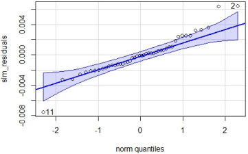
Figure 8. QQ plot of SLM residuals.
The plot displays the quantiles of the residuals plotted against the quantiles of a standard normal distribution. Ideally, if the residuals are normally distributed, the points should closely follow the reference line, which in this case is shown in blue. The shaded blue area represents the confidence bands, indicating the expected range for normally distributed data.
The histogram shown in Figure 9 represents the distribution of residuals from a spatial lag model (SLM).
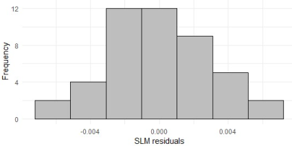
Figure 9. Histogram of residuals of SLM.
The residuals are centered around zero, with the majority values closely clustered near the center, suggesting that the model’s predictions are generally unbiased, without any systematic overestimation or underestimation. Notably, the absence of extreme outliers implies that the assumptions of normality and homoscedasticity in the residuals may hold. Although a formal statistical test would be necessary to confirm this, the visual assessment suggests that the residuals are evenly distributed around zero, enhancing confidence in the model’s reliability.
The scatter plot of residuals for the Spatial Lag Model (SLM), shown in Figure 10, illustrates the relationship between the residuals, which are the differences between the observed and predicted values, and the fitted values. Analyzing the residuals helps identify patterns that may indicate model misspecification, such as spatial autocorrelation or heteroscedasticity.
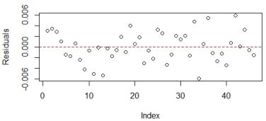
Figure 10. Residual of SLM scatter plot.
From the plot, we observe that the residuals are randomly scattered around the horizontal line at zero. This random distribution suggests that the model does not exhibit any obvious pattern in the residuals, reinforcing the likelihood that the assumptions of linearity and homoscedasticity are satisfied. The absence of any discernible trends further confirms that the model is not affected by significant issues related to heteroscedasticity or non-linearity.
The results from the Moran I test, as presented in Table 8, reveal a Moran I statistic of 0.0489, indicating minimal spatial autocorrelation in the residuals. This interpretation is further supported by the p-value of 0.2272, which is above the commonly accepted significance threshold of 0.05. Therefore, we fail to reject the null hypothesis of no spatial autocorrelation in the residuals.
Table 8. Moran I Test Results.

Statistic

Value

Sample estimate: Moran I statistic

0.0482

Moran I statistic standard deviate

0.7482

p-value

0.2272

Expectation

-0.02222

Variance

0.0087

The results provide confidence in the model’s ability to account for spatial dependence within the data.
4. Discussion
This study provides valuable insights into the spatial distribution of cardiovascular disease (CVD) prevalence in Kenya, revealing distinct regional patterns. Notably, counties such as Nyeri, Murang’a, Kirinyaga, and Embu emerged as CVD hotspots, characterised by significant clustering of CVD cases. These findings corroborate earlier research, which attributes such clustering to regional heterogeneity in environmental, socioeconomic, and behavioral determinants of health . In contrast, counties such as Wajir, Garissa, and Marsabit exhibit lower prevalence of CVD.
Physiological factors such as high body mass index, a widely accepted marker of overweight and obesity, featured prominently having a direct and significant association with CVD risk. This finding is consistent with previous studies , which identified diabetes as a major predictor of CVD morbidity and mortality, particularly in the context of ischemic heart disease and stroke. These results highlight the necessity for community-level interventions targeting obesity prevention through improved nutrition, increased physical activity, and health education on the risks of excess body weight.
Behavioral risk factors, particularly high use of tobacco, emerged as key contributors to CVD risk. The harmful chemicals introduced into the bloodstream through smoking and tobacco use have direct and indirect detrimental effects on cardiovascular health. These findings echo the conclusions of previous research, which identified tobacco control as a critical public health priority in Kenya . The evidence calls for intestified antitobacco policies, public education campaigns, and cessation support services.
An intriguing aspect of the analysis was the role of population density on the risk of CVD. Counties with high population density tend to report slightly higher CVD prevalence, likely attributed to environmental stressors such as air pollution. Interestingly, the study observed that high urbanization rates are correlated with lower prevalence of CVD, a finding that contrasts with earlier research which reported increased CVD risks in highly urbanized regions . This discrepancy highlights the complexity of urban health dynamics in Kenya and suggests that urbanization may offer protective benefits through better access to healthcare and health promotion services, a relationship that warrants further investigation.
Economic disparities were also evident in the spatial distribution of CVD. The Gross County Product (GCP), a measure of local economic performance, exhibited a significant inverse association with the CVD prevalence. This association is consistent with earlier research findings . The study finds that high alcohol use to be associated with a lower risk of CVD, despite the known adverse effects of excessive consumption. A systematic review and meta-analysis reported a reduced risk of heart failure associated with moderate alcohol consumption in community settings . The present findings echo this complex relationship but caution is warranted, as the threshold between beneficial and harmful consumption remains poorly defined. and requires further research. Finally, the study explored dietary risks where higher dietary risks were associated with higher CVD prevalence supporting the conventional assumptions about diet and heart health.
Future efforts should prioritize strengthening health data systems to address the persistent gaps in CVD reporting, particularly in remote and underserved regions of Kenya. Enhanced collaboration between the Ministry of Health (MOH), the Kenya Health Information System (KHIS), and innovative health data platforms such as Signalytic is essential for improving the quality, timeliness, and representative of health data to support evidence-based decision-making. By investing in robust, inclusive data collection and analysis frameworks, Kenya can improve public health planning, reduce regional disparities, and enhance the effectiveness of national cardiovascular disease prevention strategies.
5. Conclusion
This study reveals significant spatial disparities in the prevalence of cardiovascular disease (CVD) across Kenya, shaped by a complex interplay of physiological, behavioral, and socioeconomic factors. Strengthening health information systems and improving data quality, particularly in undeserved and remote areas, remains crucial to achieving equitable health outcomes. Partnerships between the Ministry of Health (MOH), Kenya Health Information System (KHIS), and health data innovators may offer valuable opportunities to close data gaps and support evidence-based policy-making.
A comprehensive approach that integrates health promotion, economic support, expanded access to healthcare, more comprehensive approach to data collection and further research is critical in addressing the complex drivers of CVD in Kenya.
Abbreviations

CVD

Cardiovascular Disease

GBD

Global Burden of Disease

GCP

Gross County Product

HBMI

High Body Mass Index

HBP

High Blood Pressure

KNBS

Kenya National Bureau of Statistics

LM

Lagrange Multiplier

NCD

Non-Communicable Diseases

SAR

Spatial Autoregressive

SDM

Spatial Durbin Model

SEM

Spatial Error Model

SR

Standardized Rate

WHO

World Health Organization

Acknowledgments
I extend my sincere appreciation to all individuals and institutions whose support made this research possible. I am particularly grateful to my academic supervisor and mentors for their invaluable guidance, constant feedback, and continuous encouragement throughout the study. I also acknowledge the contributions of stakeholders and organizations that facilitated access to essential data and resources, enabling the development and validation of the models presented. Lastly, I express deep gratitude to my family, friends, and colleagues for their unwavering support and encouragement, which were instrumental in the successful completion of this cardiovascular disease research.
Author Contributions
Grace Wanjiku Mwangi: Conceptualization, Data curation, Formal Analysis, Methodology, Resources, Visualization, Writing – original draft
Anthony Kibira Wanjoya: Conceptualization, Supervision, Writing – review & editing
Conflicts of Interest
The authors declare no conflicts of interest.
References
[1] World Health Organization, ”Cardiovascular diseases”. (2021). Available from:
[2] Mensah, G. A., Roth, G. A., & Fuster, V. (2019). The global burden of cardiovascular diseases and risk factors: 2020 and beyond. Journal of the American College of Cardiology, 74(20), 2529-2532.
[3] Ministry of Health, “Kenya STEPwise Survey for Non-Communicable Diseases Risk Factors 2015 Report”. Available from:
[4] Mbau, L., Fourie, J. M., Scholtz, W., Nel, G., Scarlatescu, O., & Gathecha, G. (2021). PASCAR and WHF Cardiovascular diseases Scorecard project. Cardiovascular Journal of Africa, 32(3), 161-167.
[5] Moraga, P. (2023). Spatial statistics for data science: theory and practice with R. CRC Press.
[6] Zhang, C. (2012). Spatial weights matrix and its application. Journal of Regional Development Studies, 15, 85-97.
[7] Zhou, X., & Lin, H. (2008). Spatial weights matrix. In S. Shekhar & H. Xiong (Eds.), Encyclopedia of GIS (pp. 1113-1113). Springer US.
[8] Shekhar, S., Xiong, H., & Zhou, X. (Eds.). (2017). Encyclopedia of GIS (2nd ed.). Springer International Publishing.
[9] Environmental Systems Research Institute. (2021). ArcGIS Pro (Version 2.8) [Computer software].
[10] Elhorst, J. P. (2014). Spatial econometrics: from crosssectional data to spatial panels (Vol. 479, p. 480). Heidelberg: Springer.
[11] Yamagata, Y., & Seya, H. (Eds.). (2019). Spatial analysis using big data: Methods and urban applications. Academic Press.
[12] Ruttenauer, T. (2022). Spatial regression models: a systematic comparison of different model specifications using Monte Carlo experiments. Sociological Methods & Research, 51(2), 728-759.
[13] Florax, R. J., Folmer, H., & Rey, S. J. (2003). Specification searches in spatial econometrics: the relevance of Hendry’s methodology. Regional science and urban economics, 33(5), 557-579.
[14] Grekousis, G. (2020). Spatial analysis methods and practice: describe-explore-explain through GIS. Cambridge University Press.
[15] Addie, O., & John Taiwo, O. (2024). Predictors of diagnosed cardiovascular diseases and their spatial heterogeneity in Lagos State, Nigeria. Open Health, 5(1), 20230018.
[16] Dwane, N., Wabiri, N., & Manda, S. (2020). Small-area variation of cardiovascular diseases and select risk factors and their association to household and area poverty in South Africa: Capturing emerging trends in South Africa to better target local level interventions. PLoS One, 15(4), e0230564.
[17] Darikwa, T. B., & Manda, S. O. (2020). Spatial co-clustering of cardiovascular diseases and select risk factors among adults in South Africa. International Journal of Environmental Research and Public Health, 17(10), 3583.
[18] Baptista, E. A., & Queiroz, B. L. (2022). Spatial analysis of cardiovascular mortality and associated factors around the world. BMC public health, 22(1), 1556.
[19] Yoon, S. J., Jung, J. G., Lee, S., Kim, J. S., Ahn, S. k., Shin, E. S., Jang, J. E., & Lim, S. H. (2020). The protective effect of alcohol consumption on the incidence of cardiovascular diseases: Is it real? A systematic review and meta-analysis of studies conducted in community settings. BMC Public Health, 20, 1-9.
[20] Roth, G. A., Johnson, C. O., Abate, K. H., AbdAllah, F., Ahmed, M., Alam, T., & Murray, C. J. L. (2017). Trends and patterns of geographic variation in cardiovascular mortality among US counties, 1980-2014. JAMA, 317(19), 1976-1992.
[21] Zangeneh, A., Amini, S., Khalili, D., Fattahi, N., Shafiee, A., & Fotouhi, A. (2024). Epidemiological patterns and spatiotemporal analysis of cardiovascular disease mortality in Iran: Development of public health strategies and policies. Current Problems in Cardiology, 49(8), Article 102675.
[22] Wang, Y., Chen, X., & Xue, F. (2024). A review of Bayesian spatiotemporal models in spatial epidemiology. ISPRS International Journal of Geo-Information, 13(3), Article 97.
[23] Fabiyi, O. O., & Garuba, O. E. (2015). Geo-spatial analysis of cardiovascular disease and biomedical risk factors in Ibadan, South-Western Nigeria. Journal of Settlements and Spatial Planning, 6(1), 61-69.
[24] Kandala, N.-B., Gebremedhin, G., Tlou, B., Koyanagi, A., Manda, S., & Lakew, Y. (2021). Mapping the burden of hypertension in South Africa: A comparative analysis of the national 2012 SANHANES and the 2016 Demographic and Health Survey. International Journal of Environmental Research and Public Health, 18(10), 5445.
[25] Mwenzwa, E. M., & Misati, J. A. (2014). Kenya’s social development proposals and challenges: Review of Kenya Vision 2030 first medium-term plan, 2008-2012.
[26] Asiki, G., Kyobutungi, C., Ezeh, A., Joshi, M. D., Oti, S., & Awuor, C. (2018). Policy environment for prevention, control and management of cardiovascular diseases in primary health care in Kenya. BMC Health Services Research, 18(1), 1-9.
[27] Global Burden of Disease Collaborative Network (2022). Global Burden of Disease Study 2021 (GBD 2021) results. Seattle, United States: Institute for Health Metrics and Evaluation (IHME).
[28] Kenya National Bureau of Statistics. (2023). 2019 Kenya Population and Housing Census: Volume IV- Distribution of population by socio-economic characteristics.
Cite This Article
  • APA Style

    Mwangi, G. W., Wanjoya, A. K. (2026). Spatial Modeling of Cardiovascular Disease in Kenya. American Journal of Theoretical and Applied Statistics, 15(2), 59-71. https://doi.org/10.11648/j.ajtas.20261502.14

    Copy | Download

    ACS Style

    Mwangi, G. W.; Wanjoya, A. K. Spatial Modeling of Cardiovascular Disease in Kenya. Am. J. Theor. Appl. Stat. 2026, 15(2), 59-71. doi: 10.11648/j.ajtas.20261502.14

    Copy | Download

    AMA Style

    Mwangi GW, Wanjoya AK. Spatial Modeling of Cardiovascular Disease in Kenya. Am J Theor Appl Stat. 2026;15(2):59-71. doi: 10.11648/j.ajtas.20261502.14

    Copy | Download

  • @article{10.11648/j.ajtas.20261502.14,
      author = {Grace Wanjiku Mwangi and Anthony Kibira Wanjoya},
      title = {Spatial Modeling of Cardiovascular Disease in Kenya},
      journal = {American Journal of Theoretical and Applied Statistics},
      volume = {15},
      number = {2},
      pages = {59-71},
      doi = {10.11648/j.ajtas.20261502.14},
      url = {https://doi.org/10.11648/j.ajtas.20261502.14},
      eprint = {https://article.sciencepublishinggroup.com/pdf/10.11648.j.ajtas.20261502.14},
      abstract = {The study conducts an assessment of the spatial distribution of cardiovascular diseases (CVD) in Kenya by integrating spatial modeling techniques and spatial autocorrelation measures. CVDs, which refer to disorders of the heart and blood vessels, have surpassed communicable diseases as the leading cause of morbidity and mortality worldwide, posing a critical public health concern, especially in low- and middle-income countries (LMICs) where resources remain limited. A growing body of global evidence has revealed marked geographical disparities in CVD incidence, prompting investigations into small-area spatial distribution patterns. This study employed both global and local spatial autocorrelation measures to analyze CVD prevalence across Kenyan counties. The Global Moran’s I statistic was used to assess the overall degree of spatial clustering, while the Local Moran’s I identified significant clusters of high and low prevalence, alongside spatial outliers. Additionally, the Getis-Ord Gi* statistic was applied to detect statistically significant hotspots and coldspots, revealing important spatial patterns in disease prevalence. Spatial regression models were compared using the Lagrange Multiplier (LM) test, Akaike Information Criterion (AIC), and Bayesian Information Criterion (BIC) for model selection. The Spatial Lag Model (SLM) demonstrated superior performance over the Spatial Error Model (SEM) and the Spatial Durbin Model (SDM), achieving a Rao’s score (RSlag) of 16.449 and an adjusted score (adjRSlag) of 12.181, both statistically significant at the 5% level. The SLM also recorded the lowest AIC and BIC values at -380.09 and -361.80, respectively, confirming its suitability in capturing spatial dependence in the data. The findings revealed significant spatial clustering of CVD prevalence, with distinct high-risk and low-risk regions across the country. High body mass index (HBMI), tobacco use, and poor dietary habits emerged as major risk factors driving CVD prevalence, while urbanization and economic development were associated with lower disease burdens. The study highlights the importance of incorporating spatial analysis in public health planning to inform targeted interventions, optimize resource allocation, and enhance community health education campaigns aimed at promoting heart-healthy lifestyles.},
     year = {2026}
    }
    

    Copy | Download

  • TY  - JOUR
    T1  - Spatial Modeling of Cardiovascular Disease in Kenya
    AU  - Grace Wanjiku Mwangi
    AU  - Anthony Kibira Wanjoya
    Y1  - 2026/04/16
    PY  - 2026
    N1  - https://doi.org/10.11648/j.ajtas.20261502.14
    DO  - 10.11648/j.ajtas.20261502.14
    T2  - American Journal of Theoretical and Applied Statistics
    JF  - American Journal of Theoretical and Applied Statistics
    JO  - American Journal of Theoretical and Applied Statistics
    SP  - 59
    EP  - 71
    PB  - Science Publishing Group
    SN  - 2326-9006
    UR  - https://doi.org/10.11648/j.ajtas.20261502.14
    AB  - The study conducts an assessment of the spatial distribution of cardiovascular diseases (CVD) in Kenya by integrating spatial modeling techniques and spatial autocorrelation measures. CVDs, which refer to disorders of the heart and blood vessels, have surpassed communicable diseases as the leading cause of morbidity and mortality worldwide, posing a critical public health concern, especially in low- and middle-income countries (LMICs) where resources remain limited. A growing body of global evidence has revealed marked geographical disparities in CVD incidence, prompting investigations into small-area spatial distribution patterns. This study employed both global and local spatial autocorrelation measures to analyze CVD prevalence across Kenyan counties. The Global Moran’s I statistic was used to assess the overall degree of spatial clustering, while the Local Moran’s I identified significant clusters of high and low prevalence, alongside spatial outliers. Additionally, the Getis-Ord Gi* statistic was applied to detect statistically significant hotspots and coldspots, revealing important spatial patterns in disease prevalence. Spatial regression models were compared using the Lagrange Multiplier (LM) test, Akaike Information Criterion (AIC), and Bayesian Information Criterion (BIC) for model selection. The Spatial Lag Model (SLM) demonstrated superior performance over the Spatial Error Model (SEM) and the Spatial Durbin Model (SDM), achieving a Rao’s score (RSlag) of 16.449 and an adjusted score (adjRSlag) of 12.181, both statistically significant at the 5% level. The SLM also recorded the lowest AIC and BIC values at -380.09 and -361.80, respectively, confirming its suitability in capturing spatial dependence in the data. The findings revealed significant spatial clustering of CVD prevalence, with distinct high-risk and low-risk regions across the country. High body mass index (HBMI), tobacco use, and poor dietary habits emerged as major risk factors driving CVD prevalence, while urbanization and economic development were associated with lower disease burdens. The study highlights the importance of incorporating spatial analysis in public health planning to inform targeted interventions, optimize resource allocation, and enhance community health education campaigns aimed at promoting heart-healthy lifestyles.
    VL  - 15
    IS  - 2
    ER  - 

    Copy | Download

Author Information
  • Abstract
  • Keywords
  • Document Sections

    1. 1. Introduction
    2. 2. Methodology
    3. 3. Results
    4. 4. Discussion
    5. 5. Conclusion
    Show Full Outline
  • Abbreviations
  • Acknowledgments
  • Author Contributions
  • Conflicts of Interest
  • References
  • Cite This Article
  • Author Information